There are 26,000 SENSORS buried under the pavements of California freeways. Every thirty seconds, those sensors send data to our computers here in Berkeley. The data tell us about the number of cars driving on that freeway and their speed at that time. We also collect, process, and store data about collisions and other incidents. This database, PeMS (Performance Monitoring System), is now by far the most comprehensive source of information about California highways. Today it stores four trillion bytes of information, which are available online. We’ve already learned quite a lot from all those data. For example, we’ve found the error in the old belief that an average speed of 40 to 45 mph maximizes traffic capacity; we now know for a fact that maximum capacity occurs at around 60 mph. And we’ve been surprised to discover that some HOV lanes may have the perverse effect of actually adding to congestion.
We’ve learned a lot that’s proving routinely helpful on a day-to-day basis too. We’re pretty sure we can now better manage the flow of traffic and thus lessen congestion. By integrating our research findings into Caltrans’s freeway-management operations, we are helping the state DOT improve traffic behavior.
What else can we learn from PeMS data? Here’s a summary of some of the empirical knowledge about highway congestion we’ve gained from analyzing five year’s worth of PeMS data. There is still much to be learned, and many more ways the data can be analyzed and used by traffic engineers, transportation planners, policymakers, researchers, and the public.
Congestion Dynamics
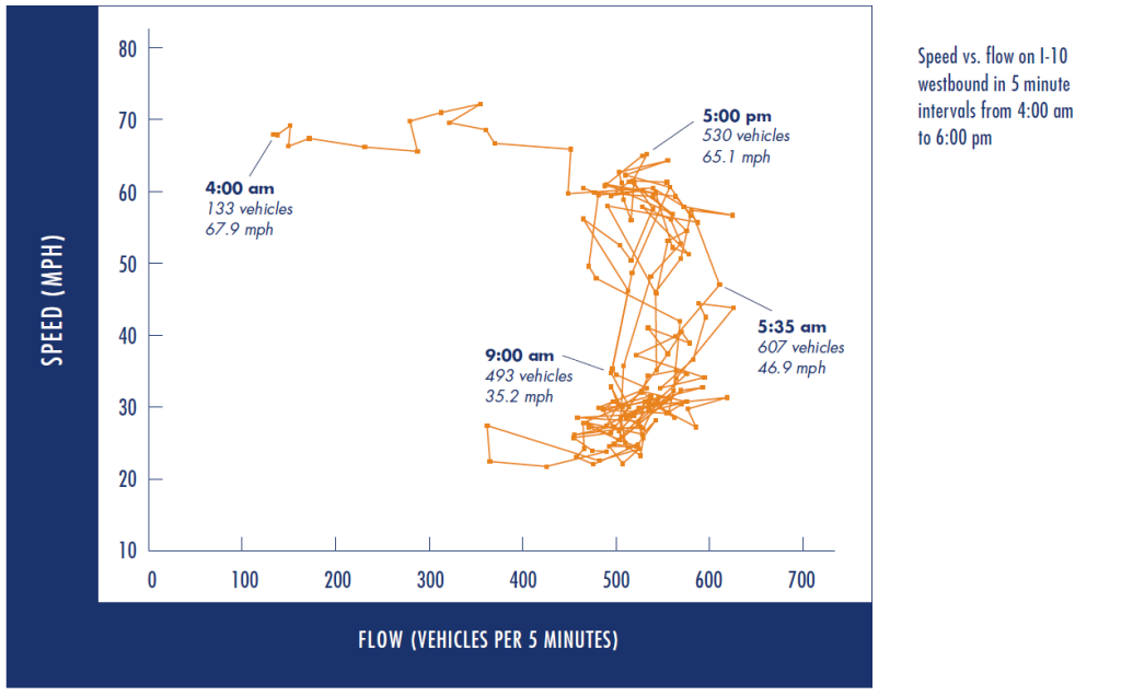 Congestion begins when traffic switches from a 60-mph, high-volume free-flow state to a chaotic, low-speed, low-volume glut of vehicles. The transition occurs when vehicle density (the number of vehicles per mile in a lane) exceeds a critical level. Once it enters the congestion state, it takes a long time for traffic to return to free-flow, and meanwhile delay accumulates. Figure 1 illustrates this phenomenon. It plots speed vs. flow at five-minute intervals across all four lanes of westbound freeway I-10 in Los Angeles. Early in the morning, speed remains at 60 mph while the flow quadruples from 150 vehicles per five-minute segment at 4:00 a.m. to a maximum of 625 vehicles at 5:35 a.m. An influx of vehicles at that point pushes vehicle density above the critical level, forcing traffic into the congestion state. At 9:00 a.m. flow is down to about 500 vehicles per five minutes and speed is much slower at about 30 mph. Traffic doesn’t return to free flow until around 5:00 p.m.
Two important implications follow from speed-flow patterns like that in Figure 1. First, the maximum flow or capacity of a freeway segment is reached while traffic is moving freely. As a result, freeways are most productive when they carry capacity flows at 60 mph; operating freeways at lower speeds always imposes additional delay.
Second, if a ramp metering policy holds back incoming vehicles so that vehicle density is kept below its critical value, traffic will flow freely and congestion will be avoided altogether. Call such a ramp-metering policy an Ideal Metering Policy or IMP. Although IMP may impose queuing delays at on-ramps, there is a net reduction in congestion delay because vehicles on the freeway move at free-flow speeds and at capacity volumes.
Bottlenecks
Bottlenecks may be caused by a physical disruption such as a reduced number of lanes, a change in grade, or an on-ramp with a short merge lane. Such bottlenecks recur predictably at the same time of day and same day of week. Nonrecurring bottlenecks are caused by collisions or highway repairs that block one or more lanes, or by special events like ball games that create demand surges, or by adverse weather that reduces capacity.
We find that nearly half of weekday, peak-period congestion delay in California occurs at 600 recurrent bottlenecks. Taking measures to mitigate the severity of just these bottlenecks would reduce congestion significantly. An additional 28 percent of the peak-period congestion delay is caused by collisions, with 10 percent of it accounting for 90 percent of all collision-induced delay. Rapid detection and clearance of these worst collisions would further reduce congestion.
Ramp Metering
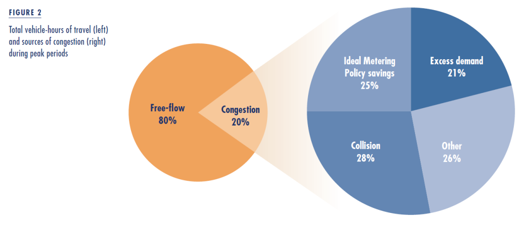 As stated above, if traffic were controlled so that vehicle density never exceeds a critical value, congestion could be avoided altogether. Large volume surges at on-ramps can often cause traffic numbers to exceed this critical value. An Ideal Metering Policy (IMP) would prevent these surges and maintain freeway traffic in free-flow state, although at the cost of queuing delay on the ramps. With IMP, freeway traffic flows at capacity, so when demand exceeds capacity, vehicles must queue up. Recall that half of all delay is caused by 600 recurrent bottlenecks. Applying IMP at these bottlenecks alone would yield a net savings in delay equal to 25 percent of all congestion delay. Excess demand would move 21 percent of the congestion delay to on-ramps.
The two pie charts of Figure 2 summarize these estimates. During peak periods, motorists spend twenty percent of their time in congestion. A quarter of this delay could be saved by appropriate ramp metering; collisions cause 28 percent; and excess demand creates 21 percent of total peak-period demand.
Travel-Time Advice
 Congestion increases both average travel time and its uncertainty. Real-time data collected by PeMS can accurately predict travel time and thus reduce uncertainty. Making these predictions available to travelers through websites and telephone services like 511 can provide large benefits, virtually without cost. Accurate predictions can, over time, alter trip patterns in ways that reduce total congestion.
If predictions are available for alternative routes, a traveler can select the one with the shortest predicted travel time. Table 1 lists statistics for five origin-destination pairs in Southern California, each with alternative routes. The shortest route is predicted in two ways. A historical predictor recommends the route that in the past has had the shortest average travel time at the desired time of day. (An experienced commuter would automatically select this route.) A real-time predictor recommends the route that is expected to be shortest based on real-time data, that is, on what is actually happening until this moment. In all five examples, real-time prediction is better than historical prediction. PeMS data can provide real-time estimates with high precision. The column Travel Time Reduction shows how much average travel time improves when using real-time prediction.
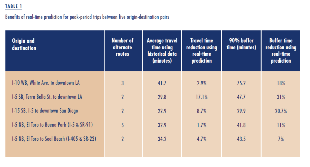 Even more significant to travelers is the reduction in travel time uncertainty. We measure this using what we call the ninety percent buffer time, or the amount of time a traveler needs to set aside to be ninety percent sure of reaching the destination on time. As expected, the buffer time is much larger than the average travel time. A real-time predictor achieves large savings in buffer time compared with a historical predictor, as indicated in the last column of Table 1.
HOV Lanes
A high-occupancy-vehicle (HOV) restriction reduces congestion by encouraging carpooling. But it also increases congestion in two ways. First, the restriction imposes a non-HOV congestion penalty by increasing congestion on the non-HOV lanes. Second, it imposes an HOV capacity penalty by decreasing the capacity of the HOV lane itself. Analysis of Bay Area data suggests that the effect of the combined penalties is larger than the positive carpooling effect. Thus, the likely net result of HOV restrictions in the Bay Area is worsening congestion.
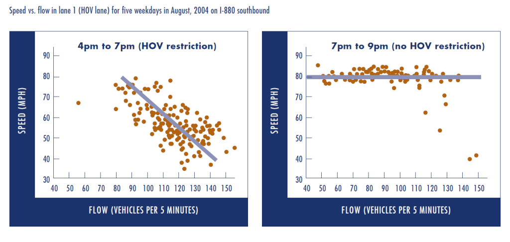 Bay Area data facilitate such assessments because the area’s HOV lanes are time limited (5:00 to 9:00 a.m. and 3:00 to 7:00 p.m.), allowing us to compare traffic on the same freeway segments during and outside of HOV restriction periods. Figure 3 helps illustrate the HOV capacity penalty. Like Figure 1, it plots speed vs. flow in lane 1 (the fast lane) in five-minute segments on southbound freeway I-880. The plot on the left is for 4:00 to 7:00 p.m., when this lane is restricted to vehicles with two or more occupants; the plot on the right is for 7:00 to 9:00 p.m., when there is no HOV restriction. The difference between the two behaviors is striking: both record maximum flow of about 145 vehicles per five-minute segment, or 1740 vehicles per hour. But, at this flow, the average speed during HOV restriction is below 50 mph (almost the same as in the non-HOV lanes), whereas the average speed outside HOV-restricted hours is nearly 80 mph.
 Another way of viewing this is to observe that the maximum flow at 60 mph during HOV restriction is 110 vehicles per five minutes, while outside HOV restriction times, maximum flow is 140 vehicles per five minutes. That is, HOV restriction at this location leads to a 21 percent capacity penalty. The capacity penalty is imposed because from 4:00 to 7:00 p.m. the HOV lane becomes a one-lane highway whose speed is governed by low-speed vehicles—the “snails” out in front. Since the non-HOV lanes are congested, an HOV vehicle wanting to go faster cannot pass a snail in front of it. The number of snails increases as HOV flow increases, causing a steep decline in speed, shown on the left of Figure 3. However, as soon as HOV restriction ends, slower drivers move to the outer lanes, and the fastest drivers move to what was the HOV lane, seen on the right of Figure 3.
Capacity estimates of non-HOV lanes at free-flow are in the range of 2,000–2,200 vehicles/lane/hour. By these estimates HOV lanes in the Bay Area are underutilized, because the number of HOVs using the lanes is on the order of 1,600 vehicles/hour, as we see in Figure 3 and from data for other HOV lanes in the Bay Area. This creates an interest in utilizing the excess capacity by converting HOV lanes to HOT (High Occupancy/Toll) lanes. However, if we take the HOV capacity penalty into account, there is very little room for additional traffic, so even cautious estimates for revenue enhancement in the Bay Area are overly optimistic. Recent legislation permitting hybrid vehicles into HOV lanes will almost certainly increase congestion.
The non-HOV congestion penalty can be illustrated with the help of Figure 4, which compares flows and speeds in left-most lanes 1 and 2 at the same location as in Figure 3. Until 3 p.m., before the HOV restriction begins, the two lanes have the same flow and approximately the same speed. When the HOV restriction begins at 3 p.m., flow in lane 1—now the HOV lane—drops dramatically, and lane 2 flow increases by the same amount. Lane 2 enters the congestion state at 3:45 p.m. with the characteristic rapid decline in flow and speed. The congestion state is caused in part by the non-HOV congestion penalty and in part by excess demand. Observe the steady decline in HOV lane speed from 4:00 to 6:30 p.m. (lower chart) because of the HOV capacity penalty. When the HOV restriction is lifted at 7:00 p.m., speed in both lanes increases dramatically: the snails move to the rightmost lanes and the faster vehicles move to the left lanes.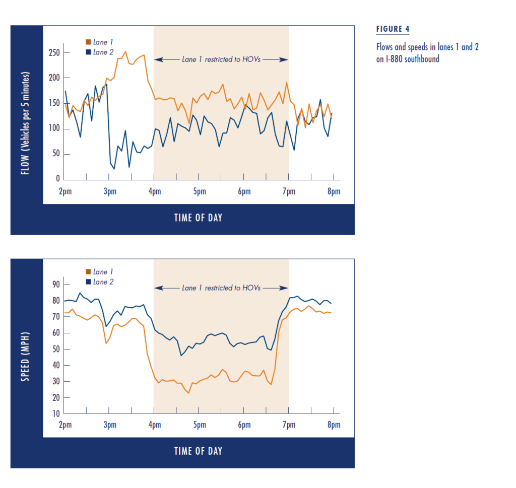
From evidence of the kind shown in Figures 3 and 4 one may confidently conclude that HOV restrictions in the Bay Area reduce total vehicle-miles traveled, increase congestion delay for non-HOV vehicles, and reduce congestion delay for HOV vehicles. To determine whether the total congestion delay is increased or reduced, we would need to know the average vehicle occupancy in HOV and non-HOV lanes at different times of day. Unfortunately occupancy estimates for the Bay Area vary significantly. Estimates at one extreme imply that HOV restrictions reduce the total number of person-miles traveled; estimates at the other extreme imply HOV lanes slightly increase this number.
 Conclusion
Congestion consumes twenty percent of the time people spend on California freeways during peak periods. Congestion will increase by ten percent per year, if we assume that travel demand will grow at a rate of two percent in the absence of effective congestion mitigation measures. Designing such measures requires a quantitative understanding of the contribution of the different causes of congestion. This review has summarized the ways that PeMS data are used now to study congestion from different perspectives, ranging from identification of bottlenecks to evaluating the benefits of ramp metering and the effectiveness of HOV lanes. Each study measures the severity of congestion and suggests approaches to its mitigation.
Further Readings
Chao Chen and Pravin Varaiya, “Max Flow in D12 Occurs at 60 mph, October 2001; Maximum Throughput in LA Occurs at 60 mph, January 2001.”
Chao Chen, et al, “Systematic Identification of Freeway Bottlenecks,” Proceedings of 83rd Transportation Research Board Annual Meeting, 2004, Washington, D.C.
Chao Chen, et al, “A System for Displaying Travel Times on Changeable Message Signs,” Proceedings of 83rd Transportation Research Board Annual Meeting, 2004, Washington, D.C.
DKS Associates. 2002 High Occupancy Vehicle (HOV) Lane Master Plan Update. March 2003.