This year Congress will draft legislation to authorize more than $120 billion in federal spending for highways, transit, and other surface transportation programs for the next six years. A critical issue is how to divide among the fifty states the Federal Highway Trust Fund revenues, which come from federal gasoline taxes and other transportation-related taxes. For the past forty years, apportioning trust fund revenues has been analogous to dividing a transportation pie among the states. With the Interstate highway program completed, Congress must now determine how much each state should receive from the trust fund, compared to what it pays in.
Dividing the Federal Transportation Pie
The popular image has Congress distributing funds on purely political bases. Amusing stories of “pork-barrel” projects suggest that powerful committee members direct public-works funds to their own districts. Yet, while the number of specifically earmarked federal transportation projects has risen over the past twenty years, these projects are not as significant as popular accounts may suggest. Earmarked funding included in the 1991 surface transportation legislation amounted to $6.2 billion, only 5 percent of total authorized spending.
Congress has historically apportioned most transportation funds among the states not by earmarking but through distribution formulas. These formulas, negotiated during the legislative process, have historically assigned funds to the states based on measurable factors such as land area, population, mileage of federal-aid highways, vehicle miles-of-travel, and cost estimates of highway construction. The funding formulas have determined the size of each state’s portion of the transportation pie.
Earmarked projects are like the whipped cream on the top of the pie – they attract much attention (and may taste particularly sweet to some), but they are insignificant when compared to the size of the whole pie. Some states’ portions may include much whipped cream covering a relatively narrow slice of pie. Other states may get little or no whipped cream, but receive the largest servings of pie.
These formulas, negotiated during the legislative process, have historically assigned funds to the states based on measurable factors such as land area, population, mileage of federal-aid highways, vehicle miles-of-travel, and cost estimates of highway construction.
From 1956 to 1987, the most active period of Interstate construction, federal transportation apportionment formulas did not consider the geographic sources of tax revenues. The states with the highest proportion of the nation’s motor-fuel consumption contributed most to the highway trust fund, but they did not necessarily have the greatest share of either land area or highway mileage. As a result, the share of taxes from each state has differed from the share of funds apportioned to each.
As long as all fifty states and most congressional districts gained new highway construction financing through the Interstate program, legislators focused on the benefits rather than the costs of the federal transportation pie. As the Interstate system neared completion, however, benefits of current funding became less apparent, and legislative concern over tax costs increased. It was as if all states were happy as long as each had some pie to eat. But, once some states had consumed their portions, they reconsidered how much they had to pay out to get their share the next time around.
Paying the Transportation Bill
When an early version of the Intermodal Surface Transportation Efficiency Act of 1991 (ISTEA) reached the Senate floor in the summer of 1991, disagreements over how best to divide the transportation funding pie threatened to block the bill’s approval. Some strong critics of the funding distribution were senators from “donor” states – those that had historically contributed more to the Federal Highway Trust Fund than they had received in federal apportionments.
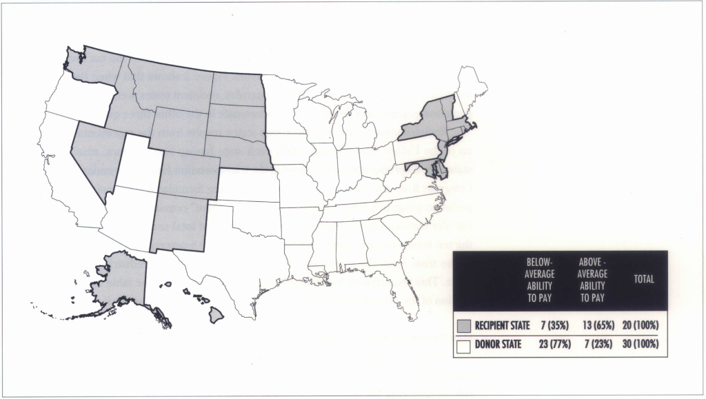
Figure 1 shows that Federal Highway Trust Fund apportionments resulted in thirty “donor” states and twenty “recipient” states in fiscal year 1991. Since donor state senators held a majority of votes, they could block ISTEA’s passage if their criticisms were not answered. The final legislation included an “equity adjustment” that guaranteed each state a minimum annual funding authorization equal to 90 percent of its trust fund contributions. The 90 percent “minimum return” guarantee helped break the 1991 legislative logjam.
Today, donor-state representatives continue to be concerned over the proportion of their trust fund contributions returned as funding authorizations. One group of states known as the “STEP 21” coalition has proposed increasing the guaranteed minimum return to 95 percent. By insuring that states receive almost all trust fund contributions back, the donor states focus attention on payments into the transportation pie. As the minimum return nears 100 percent, a state would need to provide more taxes to the Trust Fund if it is to substantially increase its portion of the federal transportation pie. An extremely high minimum return means each state would receive in apportionments an amount nearly equal to its contribution. Such a financing system would replace the single, unified federal trust fund with fifty federally administered state trust funds.
Redistribution to the Least-Populous States
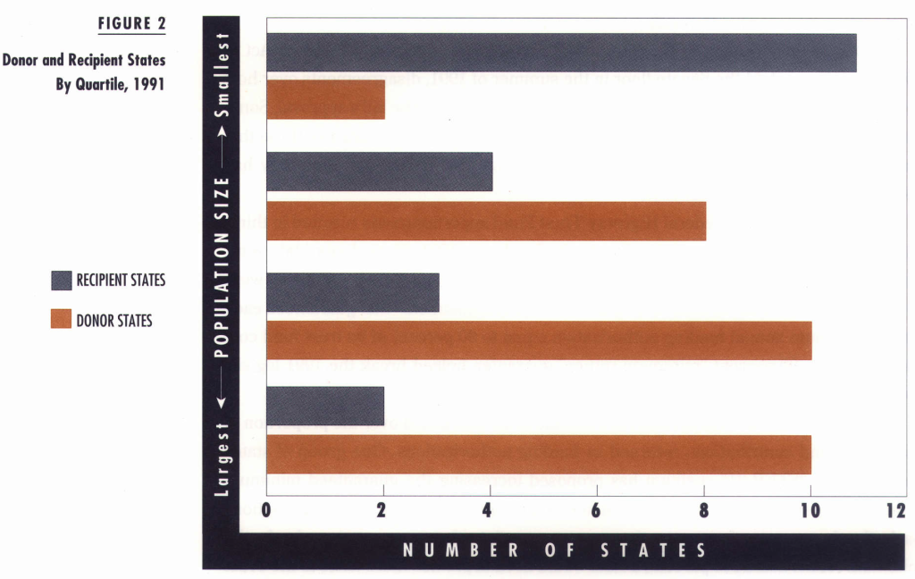
Why would such a system of separate state accounts be preferable to the earlier model of sharing a single federal account? My analysis of geographic redistribution compares state contributions to apportionments and shows which states subsidized others prior to ISTEA For fiscal year 1991 – the year before ISTEA’s 90 percent minimum return went into effect – approximately one in seven dollars (14 percent) of Federal Highway Trust Fund apportionment was geographically redistributed. Redistribution resulted when a small group of the least-populous states received some of the tax revenues paid by a large group of the more-populous states. Figure 2 shows that when the fifty states are divided by population size into four quartiles, recipient states predominate in the least populous quartile, and donor states predominate in the other three quartiles.
Redistribution to the least-populous states results from the representational makeup of the United States Senate. With each state having two senators, small-population states are disproportionately favored in the transportation-funding formulas. Members of Congress from such states can insure that funding formulas for the major federal transportation programs have a “minimum apportionment” requirement, usually that each of the fifty states receives a minimum of 0.5 percent of total annual apportionments. Since the ten least-populous states contributed less than 0.5 percent of the 1991 tax payments to the trust fund, the minimum apportionment requirement redistributes revenues to them. This requirement is analogous to giving all persons at the table a minimum-sized portion of the pie regardless how much they contribute to paying for it.
Has Federal Financing Helped the States Least Able to Pay?
It may be appropriate for the more-populous states to subsidize the least-populous states if funding is used for justifiable national purposes. One justification for the federal role in financing the Interstate highway system has been that the least-wealthy states would be unable (rather than unwilling) to pay for their Interstate segments without the federal government’s assistance. This justification is analogous to having the diners best-able to pay for their own portion of pie help pay for those who can least afford to do so. This may seem reasonable; but, in 1991 federal financing did not help the states least-able to pay.
My analysis of fiscal equalization reveals which states could best afford to pay for a portion of the pie and whether the system of geographic redistribution gives most assistance to those least able to pay. Economists commonly measure a state’s ability to raise tax revenues using the Representative Tax System (RTS) fiscal capacity. The RTS measure of revenue-raising ability uses a national average of 100, so states with RTS capacity greater than 100 have above average ability to pay and those with RTS capacity less than 100 have below-average ability to pay.
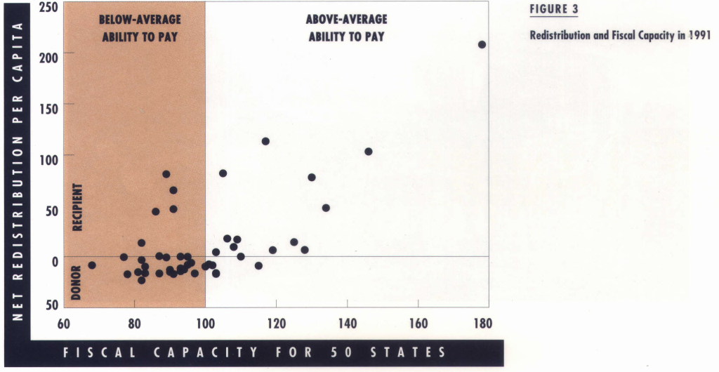
Figure 3 compares the states’ RTS fiscal capacity with the net redistribution of highway trust fund revenues per capita in fiscal year 1991. Two lines divide the figure into four quadrants, the vertical line indicating average (100) fiscal capacity and the horizontal line showing zero net redistribution of funding per capita. The table in Figure 1 summarizes the data shown in Figure 3, and shows that twenty of the fifty states were recipient states and thirty were donor states. Sixty-five percent of the recipient states have higher than average capacity; 77 percent of donor states have lower than average capacity. This means that the states that are most able to pay their own way are more often net recipients of redistribution than net donors. Meanwhile, the states least able to pay for their own shares of the pie are more often donors than recipients. This surprising outcome is analogous to a situation where the diners with below-average income subsidize the pie of the diners with above-average income, because the group has agreed to give everyone some minimum-sized portion of the pie. The generous diners may not recognize that the recipients of their subsidy may have already eaten dessert before the pie was served.
Conclusion
Proposals to give states a higher “minimum return” – up to 100 percent of their contributions – may appear self-serving, since they reduce the amount of funding available to help states with less fiscal capacity. Moreover they appear to ignore the general benefits that may result from providing transportation-related public goods, such as an increased contribution to national defense. Yet high minimum return can produce more efficient and more equitable results because states would have to raise their own revenues for transportation projects within their borders rather than use subsidies from other states.
During the year Congress passed ISTEA, many recipients of redistribution were states that could better afford to pay for their highways than could non-recipients. Proposals to increase the level of minimum return above 90 percent are consistent with recognizing that federal financing is not helping those states that most need assistance. Such proposals also recognize that incremental general benefits provided by continued federal involvement have declined substantially from the years when construction of the Interstate highway system began.
Today the fifty states seem to want the federal government to continue taxing gasoline and other transportation-related products. As a result, the states will probably continue sharing a federally administered trust fund pie. However, they’re less willing to subsidize each other’s portions of the nation’s transportation system. The logical solution is to have each state receive a portion of the pie that accurately reflects the amount of its tax bill.
Further Readings
Anderson, John E., ed., Fiscal Equalization for State and Local Government Finance, (Westport: Praeger Publishers, 1994).
Boarnet, Marlon G., “New Highways and Economic Growth: Rethinking the Link,” ACCESS, No. 7. Fall 1995, University of California Transportation Center, Berkeley.
Robert W. Poole, Jr., “Defederalizing Transportation Funding,” Policy Study No. 216, Reason Foundation, Los Angeles, 1996. United States General Accounting Office, “Federal Grants: Design Improvements Could Help Federal Resources Go Further,” Report No. GAO/AIMD-97-7, Washington, DC, 1996.
United States General Accounting Office, “Highway Funding: Alternatives for Distributing Federal Funds,” Report No. GAO/RCED-96-6, Washington, DC, 1995.