Are Americans Really Driving So Much More?

[sharelines]Vehicle miles traveled aren’t rising as fast as we thought.

Many people seem to think that increased VMT (vehicle miles traveled) spells trouble. VMT growth bothers environmentalists because it implies greater energy consumption and pollution. VMT growth concerns urban planners because it suggests increased sprawl and decreased transit use.

Both groups found plenty to worry about when the 1990 Nationwide Personal Transportation Survey (NPTS) results were published-VMT apparently grew by 41% between 1983 and 1990. But is this true?

My research develops three alternative estimates of VMT growth. All three estimates agree closely with each other, but disagree with the NPTS results. I find that VMT per vehicle grew at only half the rate indicated by the NPTS.

What made the NPTS estimates too high? Budgetary constraints forced them to use telephone surveys instead of household surveys. Internal evidence in the phone survey data shows that high-income (hence high-VMT) households were over-sampled, thus producing an overestimate for the VMT of average households.

Alternative Estimaate #1-California Odometer Survey

As my first check on the NPTS results, I developed a VMT estimate for California. The data come from California’s statewide, biennial smog-check inspections, involving nearly twenty million vehicles. Each inspection report contains the vehicle’s odometer reading and its license plate number. By matching cars across inspections, we have two odometer readings and two dates, and can compute an objective VMT rate.¹

After computing VMT for each vehicle, we aggregated the data to compute an average VMT by model-year and class (cars, light trucks, medium trucks). To compensate for any selection bias, we scaled these to state-level using the exact class and model-year distribution from vehicle registration data.

The calculated VMT growth rate for California was 1.6% per year, well below the 2.7% annual growth rate indicated by the NPTS survey. Does California’s VMT growth differ from U.S. VMT growth? Perhaps. But if it does differ, most observers would have expected California’s growth to be atypically high. Next, I turned to a nationwide sample.

Alternative Estimate #2-U.S. Department of Energy Survey

For my second check on the NPTS results, I used the U.S. Department of Energy’s Residential Transportation Energy Consumption Survey (RTECS). Only 3,000 households were surveyed. But, for purposes of VMT estimation, the RTECS data ought to have several advantages over the NPTS. The household sample comes from a national multistage probability survey, rather than from random-digit dialing; the initial interview is a personal interview in the home; and the great majority of the VMT data are based on actual odometer readings, taken about a year apart. Thus, like California’s, this survey is an objective source of VMT data. The NPTS data are subjective, based on respondent’s recollections of miles driven.

Estimates of VMT growth based on the RTECS survey are nearly identical to those based on the California data: 1.5% per year in the RTECS sample, compared with 1.6% for California, and 2. 7%, NPTS.

Alternative Estimate #3-Federal Highway Administration Data

The Federal Highway Administration (FHWA) collects VMT statistical data from the fifty states, compiles them, and publishes them in Highway Statistics. The state VMT estimates are derived from fuel-consumption data, supplemented by sample traffic counts. The states have improved the quality of these estimates over time, but they still rely heavily on estimates of parameters – for example, average miles per gallon – rather than on actual measurements. (California has an elaborate model to estimate the average miles per gallon of its vehicle fleet.)

Given the uncertainties in the data sources, I would not use these as a primary standard. But, taken in combination with the other results, they do provide a useful comparison. Estimates of VMT growth rates based on the FHW A data are nearly identical to my other estimates: 1.4% FHWA, 1.5% RTECS, 1.6% California, compared to 2.7% reported by NPTS.

Therefore, the results from analyzing three alternative data sets appear strikingly similar with one another, but show a VMT growth rate that is only about half as fast as the NPTS estimate.

Why are the NPTS Results too High?

What are the possible sources of error? First, the NPTS estimate is based on subjective data. Respondents are asked: “How many miles did you drive last year?” There are good reasons to doubt the reliability of respondents’ answers to such a subjective question concerning an activity that they do not usually consider in quantitative terms. Still, any subjectivity problem ought to be constant over time; that is, growth rates should be unbiased.

Unfortunately, severe budget pressures caused a change in methodology in 1990. All the prior NPTS data had been collected using home interviews, but in 1990 they switched to telephone interviews based on a random-digit dialing. Inherently, random digit dialing contacts a disproportionate number of high-income households: high-income households have several phones per household, while low-income households often share a phone with other households. Survey organizations use a variety of techniques to compensate for these biases, but sometimes the correction techniques are not sufficient.

Suppose the 1990 NPTS did over-sample high-income households. This would produce an overestimate of the average VMT level because high-income households travel more. Further, the effects of the upward bias in VMT level would be compounded by the change in survey methodology: To compute growth, one compares the high 1990 level to the 1983 level that was derived using the old survey methodology. That is, the change in survey methodology would account for the overestimate of VMT growth rates.

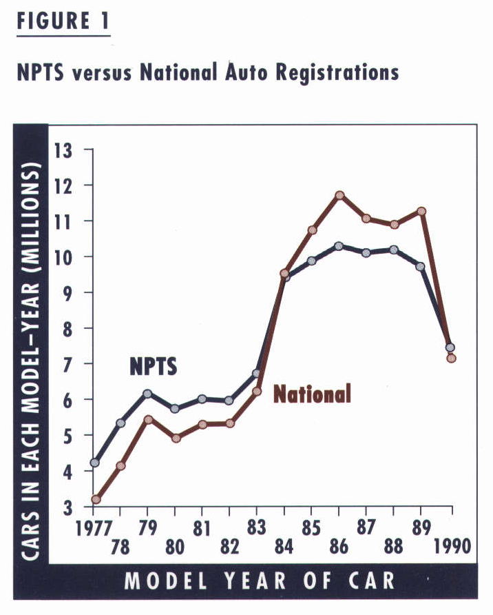
So, did the 1990 NPTS over-sample high income households? I cannot test this directly, but I devised a powerful indirect test. High-income households tend to own newer cars than do low-income households. So I computed the age distribution (model-year) of vehicles in the NPTS sample and compared it to the correct age distribution based on complete state vehicle registration data. Figure 1 shows the results. The dark line shows the correct age distributions. The colored line shows the distribution of the vehicles sampled by the NPTS. Clearly, the NPTS sample includes too many young cars and too few old ones.²

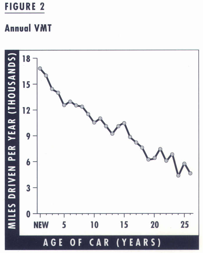
What are the consequences of oversampling new vehicles in the NITS? Figure 2 shows the relationship between vehicle age and yearly VMT: As vehicles age they are driven significantly less. Since the average car in the 1990 NPTS is newer than it ought to be, the 1990 NPTS will overestimate VMT per vehicle.

Conclusion

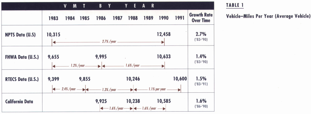
Table 1 summarizes the VMT estimates from the four data sets. The table shows the VMT per year estimates and the year to which they apply. On the right side of the table are the growth rates for the longest period applicable to each data set. Where intermediate points were available, they are shown, and the intermediate growth rates are also calculated.

The FHW A data, the RTECS data, and the California data are in close agreement on VMT per year: 10,633 miles/year, 10,600 miles/year, and 10,585 miles/year, respectively. These VMT estimates are well below the NPTS estimate of 12,458 miles/year. The FHWA, RTECS, and California estimates also give consistent estimates for overall VMT growth rates: 1.4%, 1.5%, and 1.6%, respectively. These growth rate estimates are about half the NPTS estimate.

But truth is not simply based on a three to one vote. The RTECS and California data sets are inherently higher quality than the NPTS because they collect objective odometer data. The NPTS is based on subjective VMT estimates and there was a critical change in sampling methods between 1983 and 1990. The 1990 NPTS survey used random-digit dialing, instead of home interviews, resulting in significant over-sampling of late-model, high-VMT vehicles.³

That is, there are a number of strong reasons to reject the apparent VMT jump in the 1990 NPTS. The best estimate of VMT growth for households in the 1983- 1990 period is 1.4 to 1.6% per year.

Acknowledgements

Dan Near provided critical assistance with the California odometer data; Steve Gould and David Amlin provided encouragement and advice; and Phil Wilson provided the original inspiration. Dwight French and Ronald Lambrecht gave significant assistance with the RTECS data. Alan Pisarski, Susan Liss, Pat Hu, and Ami Glazer gave advice and support. Anita Iannucci provided invaluable computer assistance.

Footnotes:

Through simple in principle, the actual matching process involved considerable effort. To assure accuracy, we used only those matches where the license plate, and model year, and make of the car were identical across the time period. Instances of broken odometers (0 VMT) were discarded, and recording errors were screened out. Identical screening procedures were applied to all years, thus any bias created by our screening is constant over time and will not affect estimates of growth rates.
Figure 1 plots only the distributions for cars. But we know that U.S. households also purchase large numbers of light trucks and that they use them in much the same way they use cars. Did the NPTS also over-sample young trucks? I don’t have the complete registration data for California’s light trucks. I plotted a version of Figure 1 for actual California light trucks versus the NPTS sample of California light trucks. It shows the same age bias.
This sampling problem will not affect many other NPTS results. Comparisons of VMT between well-specified sub-groups will be reasonable, as will be result on travel patterns, destinations, and characteristics.