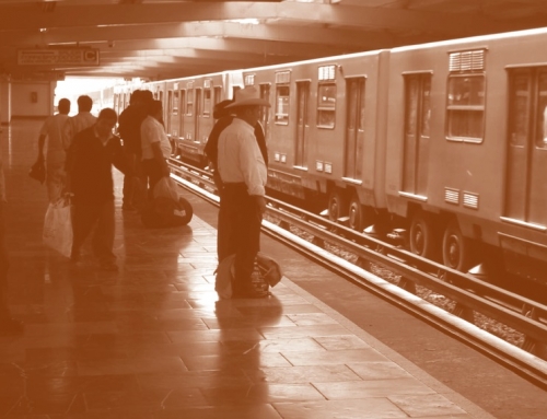
William Vickrey is the “father of congestion pricing” and a Nobel Laureate in economics. While watching the ebb and flow of traffic from his Manhattan office, he developed a hypothesis that the dynamics of rush-hour traffic have the same properties as water flowing into and out of a hypothetical bathtub.
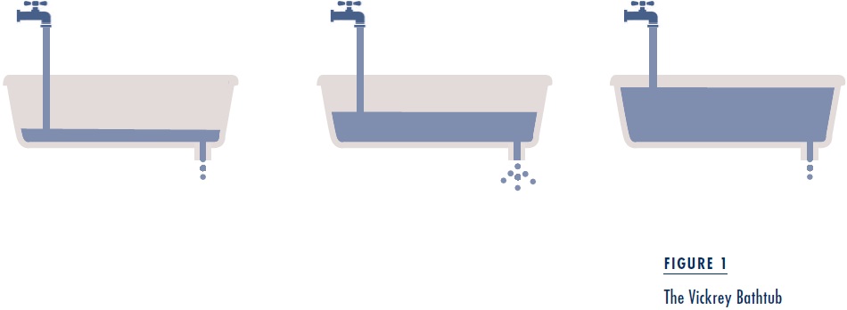
The Vickrey bathtub corresponds to Manhattan, water flowing into the bathtub corresponds to vehicles entering the traffic stream, and water draining out of the tub corresponds to vehicles exiting the stream. The height of water in the tub represents traffic density. The rate at which water drains increases with the height of the water until it reaches a critical height. Above that height, the outflow decreases as shown in Figure 1. Thus, the rate at which the bathtub drains reaches a maximum at the critical height. This critical height corresponds to the density of downtown traffic at which traffic jams start to become common. Above this level, traffic jams become more severe and the exit stream slows.
A similar phenomenon occurs in electricity distribution networks. In the context of electricity distribution, overloading the system results in brownouts and eventually blackouts. In the context of downtown traffic congestion, overloading the system results in traffic jams and eventually gridlock.
Vickrey based his hypothesis on traffic flow theory and careful observation, since there were no data on the properties of traffic flow and density for an entire downtown area a quarter century ago. In this article, I review recent empirical work that supports Vickrey’s hypothesis, I report on my own work developing a formal model of the Vickrey bathtub, and I discuss how the hypothesis provides insight into managing downtown traffic congestion through pricing.
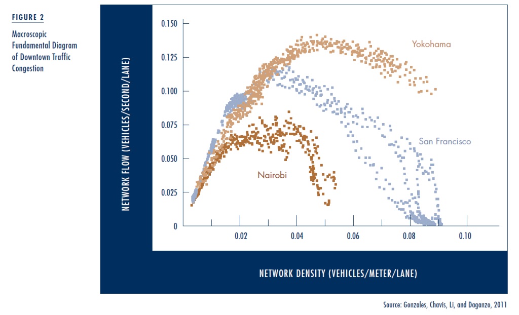
Recent work by Carlos Daganzo and his students at UC Berkeley shows a predictable relationship between traffic flow and traffic density at the scale of a downtown area. They refer to this relationship as the area’s macroscopic fundamental diagram (MFD). Figure 2 shows the MFDs for three cities around the world. Each dot corresponds to an observation. Observations were made at regular intervals throughout the business day and over days of the workweek. The observations document two important empirical regularities. First, under heavily congested conditions, traffic flow falls markedly as traffic density increases (which corresponds to the bathtub draining more slowly at high water levels). Second, the ratio of the outflow from the traffic stream to traffic flow is approximately constant (which corresponds to the bathtub draining at a rate that is tightly related to the height of water in the bathtub). Together, these two empirical regularities show that the Vickrey bathtub describes well how congested traffic behaves at the level of a downtown area. Other researchers have since confirmed these results for other cities.
Physics of Traffic Congestion
Macroscopic models of traffic flow examine the relationship between the flow, density, and speed of traffic. In contrast, microscopic models focus on the behavior of individual vehicles.
In 1935 Bruce Greenshields reported on observations he made of the speed and traffic density of cars along a section of highway. He found that speed falls linearly with increasing density, from a maximum speed at zero density to complete gridlock at jam density. This finding is now referred to as Greenshields’ Relation.
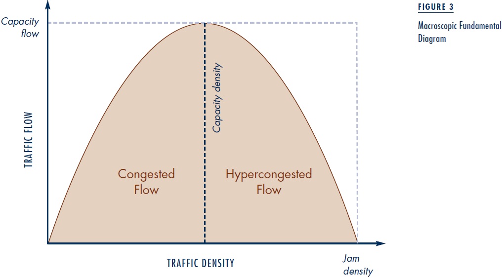
Combining Greenshields’ Relation with the fact that flow is the product of density and speed generates the MFD displayed in Figure 3. The maximum flow—known as capacity flow or simply capacity—occurs at an intermediate density, known as capacity density. Travel on the upward-sloping portion of the MFD, labeled “congested flow,” corresponds to normal congestion, where flow increases with density. Flow decreases with increasing density on the downward-sloping portion of the macroscopic diagram, labeled “hypercongested flow.”
The installation of the first loop detectors on freeways in the early 1980s generated an abundance of data, which spawned considerably more sophisticated models of freeway traffic flow. However, until the very recent work reported above, no comparable data had been collected at the scale of a downtown area, and little comparable modeling had been done for downtown traffic. To simplify my model, I assume that Greenshields’ Relation holds for downtown traffic. I also assume that the rate at which traffic exits the traffic stream is proportional to traffic flow. Together, these assumptions result in a model whose physics is analogous to that of the Vickrey bathtub.
Economics of Rush-Hour Traffic Congestion
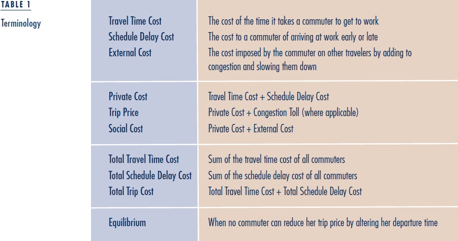
Consider a situation in which a fixed number of commuters travel from home to work over the morning rush hour. Each commuter has the same work start time and travels the same distance over city streets from home to work. Since it is physically impossible for all commuters to arrive at work exactly on time, some arrive early and others arrive late, experiencing costly schedule delay. Commuters arriving exactly on time experience no schedule delay but a large travel time cost since they travel when traffic is most congested. In contrast, commuters departing at the beginning of the rush hour experience little congestion and therefore shorter travel times, but they arrive at work considerably before their work start time, experiencing high schedule delay cost. The private cost incurred by a particular commuter equals her travel time cost plus her schedule delay cost. A commuter’s trip price equals her private cost plus the congestion toll she pays, if a toll is in place. A commuter imposes an external cost on other travelers by adding to congestion and slowing other commuters down. The social cost of a trip is the increase in total trip costs the trip causes, and equals the private cost incurred by the commuter plus the external cost the trip imposes on others.
I compare the model’s optimum morning rush-hour traffic dynamics, which can be achieved through ideal congestion pricing, with its no-toll equilibrium rush-hour traffic dynamics. Equilibrium is achieved when no commuter can reduce her trip price by altering her departure time. The optimum time pattern of departures minimizes total trip costs. Since transferring a commuter from a departure time with a higher social cost (private cost plus external cost) to a departure time with a lower social cost would reduce total trip costs, the optimum is achieved by equalizing the social cost of trips at different departure times. In contrast, the no-toll equilibrium time pattern of departure equalizes the private cost of trips at different departure times. Since the external cost of a trip at the peak of the rush hour is higher than one in the shoulders of the rush hour, the no-toll equilibrium pattern of departures entails excessive travel at the peak of the rush hour, causing the street system to become overloaded.
The optimum time pattern of departures minimizes the sum of total schedule delay cost and total travel time cost. Consider first how total schedule delay cost alone would be minimized. The fixed number of commuters traveling over the rush hour is analogous in the Vickrey bathtub to a fixed volume of water that passes through the tub. Initially the tap would be turned to maximum so that the water level rises as fast as possible, until it rises to the level at which outflow is maximized. The inflow would then be turned down so that it equals the outflow, which would keep the bathtub draining at the maximum rate. Finally, when the fixed volume of water has flowed into the tub, the tap would be turned off, leaving the remaining water to drain out. Total travel time cost, in contrast, would be minimized by having water enter the tub at a trickle, which would ensure that commuters experience virtually no traffic congestion. In the optimum scenario, the water level would never rise above the critical level where outflow is maximized.
In the no-toll equilibrium, in contrast, traffic density may exceed the flow-maximizing density over much of the morning rush hour. Demand relative to capacity is defined as the ratio of the actual flow to capacity flow. In the bathtub analogy, it is the time it would take for the fixed volume of water to drain at maximum outflow. The higher the demand is relative to capacity, the longer the rush hour. Suppose that demand is high relative to capacity, so that the rush hour lasts for a long time, causing the first commuter to experience a high schedule delay cost and thus a high trip price. In the no-toll equilibrium, the commuter who arrives at work on time experiences the same high trip price, only in the form of high travel time. If trip distance is short, this high travel time is possible only if this commuter’s average speed is low, which requires that traffic density exceed capacity density over at least a portion of the rush hour.
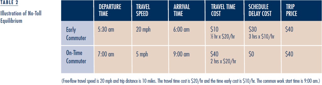
Table 2 illustrates the no-toll equilibrium in a downtown area where demand is high relative to capacity. All commuters have a work start time of 9 am and commute 10 miles from home to work on the downtown road network. Free-flow travel speed is 20 mph. Consider two commuters. The first is the earliest to depart from home and therefore the earliest to arrive at work, while the second commuter departs later and arrives exactly on time. The first commuter’s schedule delay cost is $10 for each hour she arrives early. Both commuters have a common travel time cost of $20 per hour. Demand is so high relative to capacity that the first commuter departs at 5:30 am. Traveling at close to the free-flow speed of 20 mph on the 10-mile journey to work takes slightly more than half an hour, so that she arrives at work almost three hours early. Her travel time cost is slightly above $10, and her schedule delay cost is slightly below $30, for a trip price of about $40. In the no-toll equilibrium, the commuter who arrives exactly on time must experience the same trip price of $40. Since this commuter experiences no schedule delay cost, the entire trip price must be travel time cost. Since travel time cost is $20 per hour, the journey to work takes two hours, which implies an average speed of 5 mph, only one-quarter of free-flow speed. With the assumed congestion technology, depicted in Figure 3, this low speed corresponds to heavily jammed traffic, with traffic flow substantially below capacity.
In the optimum scenario the departure rate from home is such that traffic never becomes jammed, and commuters experience only normal congestion. These optimal conditions can be achieved by charging a time-varying congestion toll set so that each commuter pays for the external cost her trip imposes on others. Each commuter’s trip price then equals the social cost of her trip. Since commuters respond to the toll by altering their departure times so that the equal trip-price condition (now including the toll) continues to be satisfied, the social cost of each trip is the same, which is the defining feature of the optimum scenario. In the example, total trip costs are so much lower when this toll is applied that, even though commuters must pay the toll, the trip price is lower than in the no-toll equilibrium. Thus, optimal tolling would still benefit commuters even if the toll revenue were completely squandered! The additional benefits from spending or redistributing toll revenue are icing on the cake.
 Building on the insights of Vickrey, I have described a model of downtown traffic congestion over the morning rush hour. This model has the property that traffic flow falls as traffic density increases beyond a critical level where traffic jams start to develop. In most large metropolitan areas, traffic jamming is severe. By reducing the incidence and severity of traffic jams, congestion tolling can improve the flow of downtown traffic during rush hours and decrease the costs of traffic congestion to such an extent that commuters are made better off even if they receive no benefits from the toll revenues collected. The strong support of the model’s properties provided by recent empirical studies of downtown traffic congestion strengthens the case for congestion tolling in practice.
This article is adapted from “A Bathtub Model of Downtown Traffic Congestion,” originally published in the Journal of Urban Economics.
Further Readings
William Vickrey. 1991. “Congestion in Midtown Manhattan in Relation to Marginal Cost Pricing,” Columbia University.